해당 자료는 전북대학교 이영미 교수님 2023고급시계열분석 자료임

CH 05, 06

1

다음의 시계열 자료 ${7, 6, 5, 8, 9, 4, 5, 5, 4, 6, 7, 8, 5, 6, 5 }$에 대하여, SACF, $\hat ρ_h (h = 1, 2, 3)$과 SPACF, $\hatϕ_{kk} (k = 1, 2)$을 직접 계산하여라. 그리고 유의수준 $α = 0.05$에서

$H_0 : ρ_h = 0 \text{vs.} H_1 : ρ_h ̸= 0$

대하여에 대한 가설검정으로 하여라.

- $\hat \rho_k$ 구하기

h=0

$Z_t= \{7, 6, 5, 8, 9, 4, 5, 5, 4, 6, 7, 8, 5, 6, 5 \}$

$Z_{t+h}= \{7, 6, 5, 8, 9, 4, 5, 5, 4, 6, 7, 8, 5, 6, 5 \}$

z = c(7, 6, 5, 8, 9, 4, 5, 5, 4, 6, 7, 8, 5, 6, 5)
mean(z)

$\bar Z_t = \bar Z_{t+h} = 6$

(z-mean(z))*(z-mean(z))

sum((z-mean(z))*(z-mean(z)))

sum((z-mean(z))*(z-mean(z)))/length(z)

2.13333333333333

$\hat Cov(Z_t- \bar Z, Z_{t+h} - \bar Z_{t+h}) = \hat Cov(Z_t- \bar Z, Z_{t} - \bar Z_{t}) = \dfrac{32}{15} = 2.1333333$

h=1

$Z_t= \{7, 6, 5, 8, 9, 4, 5, 5, 4, 6, 7, 8, 5, 6, 5, 6 \}$

$Z_{t+1}= \{6, 5, 8, 9, 4, 5, 5, 4, 6, 7, 8, 5, 6, 5, 6, 7\}$

z = c(7, 6, 5, 8, 9, 4, 5, 5, 4, 6, 7, 8, 5, 6, 5)
z1 = c(6, 5, 8, 9, 4, 5, 5, 4, 6, 7, 8, 5, 6, 5, 7)

z-mean(z)

1
0
-1
2
3
-2
-1
-1
-2
0
1
2
-1
0
-1

z1-mean(z)

0
-1
2
3
-2
-1
-1
-2
0
1
2
-1
0
-1
1

(z-mean(z))*(z1-mean(z))

0
0
-2
6
-6
2
1
2
0
0
2
-2
0
0
-1

sum((z-mean(z))*(z1-mean(z)))+1

$\hat Cov(Z_t- \bar Z, Z_{t+h} - \bar Z_{t+h}) = \hat Cov(Z_t- \bar Z, Z_{t+h} - \bar Z_{t+1})= \dfrac{3}{15}$

h=2

$Z_t= \{7, 6, 5, 8, 9, 4, 5, 5, 4, 6, 7, 8, 5, 6, 5, 6 \}$

$Z_{t+2}= \{5, 8, 9, 4, 5, 5, 4, 6, 7, 8, 5, 6, 5, 6, 7, 6\}$

z = c(7, 6, 5, 8, 9, 4, 5, 5, 4, 6, 7, 8, 5, 6, 5)
z2 = c(5, 8, 9, 4, 5, 5, 4, 6, 7, 8, 5, 6, 5, 7, 6)

(z-mean(z))*(z2-mean(z))

-1
0
-3
-4
-3
2
2
0
-2
0
-1
0
1
0
0

sum((z-mean(z))*(z2-mean(z)))+0+0

-9

$\hat Cov(Z_t- \bar Z, Z_{t+h} - \bar Z_{t+h}) = \hat Cov(Z_t- \bar Z, Z_{t+h} - \bar Z_{t+2})= -\dfrac{9}{15}$

h=3

$Z_t= \{7, 6, 5, 8, 9, 4, 5, 5, 4, 6, 7, 8, 5, 6, 5, 6 \}$

$Z_{t+3}= \{8, 9, 4, 5, 5, 4, 6, 7, 8, 5, 6, 5, 6, 7, 6, 5\}$

z = c(7, 6, 5, 8, 9, 4, 5, 5, 4, 6, 7, 8, 5, 6, 5)
z3 = c(8, 9, 4, 5, 5, 4, 6, 7, 8, 5, 6, 5, 7, 6, 5)

(z-mean(z))*(z3-mean(z))

2
0
2
-2
-3
4
0
-1
-4
0
0
-2
-1
0
1

sum((z-mean(z))*(z3-mean(z)))+1+0-1

-4

$\hat Cov(Z_t- \bar Z, Z_{t+h} - \bar Z_{t+h}) = \hat Cov(Z_t- \bar Z, Z_{t+h} - \bar Z_{t+3})= -\dfrac{4}{15}$

$\hat acf(1) = \dfrac{\hat Cov(Z_t- \bar Z, Z_{t+1} - \bar Z_{t+h})}{\hat Cov(Z_t- \bar Z, Z_{t} - \bar Z_{t+h})}=\dfrac{3/15}{32/15}=\dfrac{3}{32}$

$\hat acf(2) = \dfrac{\hat Cov(Z_t- \bar Z, Z_{t+2} - \bar Z_{t+h})}{\hat Cov(Z_t- \bar Z, Z_{t} - \bar Z_{t+h})}=\dfrac{-9/15}{32/15}=-\dfrac{9}{32}$

$\hat acf(3) = \dfrac{\hat Cov(Z_t- \bar Z, Z_{t+3} - \bar Z_{t+h})}{\hat Cov(Z_t- \bar Z, Z_{t} - \bar Z_{t+h})}=\dfrac{-4/15}{32/15}=\dfrac{-4}{32}$

rho1 = 3/32

rho2 = -9/32

rho3 = -4/32

- pacf를 구하자

$\widehat{pacf(1)} = \widehat{acf(1)} = \dfrac{3}{32}$

$\widehat{pacf(2)} = \dfrac{\rho_2 - \rho_1^2}{1-\rho_1^2}=-0.292610837438424$

pi1= 3/32

pi2=(-9/32 - (3/32)**2)/(1-(3/32)**2)

$\widehat{pacf(3)} = \dfrac{\rho_3 - \sum_{j=1}^2 \hat ϕ_{kj} \hat \rho_{3-j} }{1- \sum_{j=1}^2 \hat ϕ_{2j}\hat \rho_j}=-0.0700455193966982$

분자: $\rho_3 - \sum_{j=1}^2 \hat ϕ_{kj} \hat \rho_{3-j} = \rho_3 - \hat ϕ_{21} \hat \rho_2 - \hat ϕ_{22} \rho_1$

$\hat ϕ_{21} = \hat ϕ_{11} - \hat ϕ_{22} \hat ϕ_{11}=0.121182266009852$

pi21 = pi1-pi2*pi1

rho3 - pi21*rho2 - pi2*rho1

-0.0634852216748769

분모: $1- \sum_{j=1}^2 \hat ϕ_{2j}\hat \rho_j= 1- \hat ϕ_{21} \hat \rho_1 - \hat ϕ_{22} \hat \rho_2$

1- pi21*rho1 - pi2 * rho2

0.90634236453202

-0.0634852216748769/0.90634236453202 # rho3

-0.0700455193966982

- 유의수준 검정

$α = 0.05$에서

$H_0 : ρ_h = 0 \text{vs.} H_1 : ρ_h ̸= 0$

$\hat \rho_h > 1.96 \times \dfrac{1}{\sqrt{n}}$ 이면 기각

acf(z)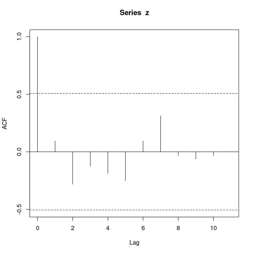

n=15
1.96*1/sqrt(n)

0.506069823904436

rho1

0.09375

rho1 > 1.96*1/sqrt(n)

FALSE

rho2

-0.28125

rho2 > 1.96*1/sqrt(n)

FALSE

rho3

-0.125

rho3 > 1.96*1/sqrt(n)

FALSE

rho1, rho2, rho3가 값보다 작으므로 기각할수 없다. 즉, rho=0이다.

2

다음의 모형들에 의해 설명되는 확률과정 $\{Z_t\}$는 정상성을 갖는가? 단 $ε_t ∼ W N(0, 1)$.

- 정상성 만족하기 위해서는

$E(Z_t) = \mu$

$Var(Z_t) = \sigma^2$

$Cov(Z_t,Z_{t+h}) = \gamma_h$

(1)

$Z_t = ε_t − ε_{t−1} − ε_{t−2}$

$E(Z_t) = E(ε_t − ε_{t−1} − ε_{t−2}) = E(ε_t)-E(ε_{t-1}) - E(ε_{t-2}) = 0$

$Var(Z_t) = Var(ε_t − ε_{t−1} − ε_{t−2}) = Var(ε_t)+Var(\epsilon_{t-1}) + Var(ε_{t−2}) = 1+1+1=3$

$\epsilon_t$는 WN이므로 $Cov(\epsilon_t, \epsilon_{t+h})=0$

$Cov(Z_t,Z_{t-h}) = Cov(ε_t - ε_{t-1} - ε_{t-2}, ε_{t-h} - ε_{t-h-1} - ε_{t-h-2})$

$\epsilon$은 WN이므로 각각 COV취해줄 수 있꼬,, 상수값 나오니까 정상 시계열 조건을 만족한다.

(2)

$Z_t = ε_tε_{t−1} + ε_{t−2}$

-> 정상시계열

$E(Z_t) = 0$

$Var(Z_t) = V(\epsilon_t \epsilon_{t-1} + \epsilon_{t-2}) = Var(\epsilon_{t-1} \epsilon_{t-2} + \epsilon_{t-3}) = V(Z_{t-1})$

$Var(Z_t) = Var(Z_{t-1}) = Var(Z_{t-2})= \dots$

$cov(Z_t, Z_{t-1}) = cov(Z_{t-1}, Z_{t-2})$

(3)

$Z_t = A sin \left( \dfrac{2}{3} πt + U \right)$, 단 A는 평균이 0이고 분산이 1인 확률변수이고, $U$ 는 상수이다.

# 필요한 라이브러리 불러오기
library(ggplot2)

# 시뮬레이션을 위한 난수 시드 설정
set.seed(123)

# 시뮬레이션 횟수
n <- 100

# A는 평균이 0이고 분산이 1인 확률변수
A <- rnorm(n, mean = 0, sd = 1)

# U는 상수
U <- 2

# 시뮬레이션된 데이터 생성
t <- seq(1, n, by = 1)
Z <- A * sin((2/3) * pi * t + U)

# 생성된 데이터 시각화
ggplot(data.frame(t, Z), aes(x = t, y = Z)) +
  geom_line() +
  labs(title = "Simulation of Z_t", x = "Time (t)", y = "Z_t")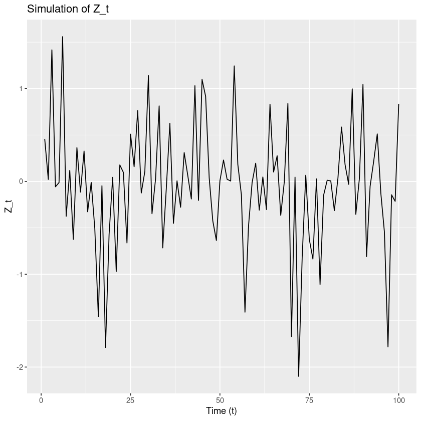

제시된 시계열 모형인 [Z_t = A (t + U)]에 대해서 정상성을 검토해보겠습니다.

주어진 모형에서 (A)는 평균이 0이고 분산이 1인 확률변수이고, (U)는 상수입니다.

평균 확인: [E(Z_t) = E(A (t + U))]

확률변수 (A)의 평균은 0이므로, [E(Z_t) = 0]

평균이 0이므로 평균 조건은 만족합니다.

분산 확인: [Var(Z_t) = Var(A (t + U))]

확률변수 (A)의 분산이 1이므로, [Var(Z_t) = Var((t + U))]

사인 함수의 범위는 -1에서 1이므로 분산은 1을 초과하지 않습니다.

[Var(Z_t) ]

분산이 상수인 경우이므로 분산 조건도 만족합니다.

공분산 확인: [Cov(Z_t, Z_{t-h}) = Cov(A (t + U), A ((t-h) + U))]

두 사인 함수는 서로 독립적이므로 공분산은 0입니다.

[Cov(Z_t, Z_{t-h}) = 0]

결론적으로, 주어진 시계열 모형도 평균과 분산이 상수이고, 공분산이 시간에 독립적이므로 정상성을 만족합니다.

(4)

$Z_t = A sin (πt + U)$, 단 $A$는 평균이 0이고 분산이 1인 확률변수이고, $U$ 는 $[−π, π]$에서의 균등분포(uniform distribution)을 따르는 확률변수이다. $A, U$ 는 서로 독립.

# 필요한 라이브러리 불러오기
library(ggplot2)

# 시뮬레이션을 위한 난수 시드 설정
set.seed(123)

# 시뮬레이션 횟수
n <- 100

# A는 평균이 0이고 분산이 1인 확률변수
A <- rnorm(n, mean = 0, sd = 1)

# U는 [-π, π]에서 균등분포를 따르는 확률변수
U <- runif(n, min = -pi, max = pi)

# 시뮬레이션된 데이터 생성
t <- seq(1, n, by = 1)
Z <- A * sin(pi * t + U)

# A는 평균이 0이고 분산이 1인 확률변수
set.seed(1)
A <- rnorm(n, mean = 0, sd = 1)

# U는 [-π, π]에서 균등분포를 따르는 확률변수
U <- runif(n, min = -pi, max = pi)

# 시뮬레이션된 데이터 생성
t <- seq(1, n, by = 1)
Z <- A * sin(pi * (t) + U)

Z1 <- A * sin(pi * (t+4) + U)

set.seed(1)
cov(Z, Z1)

0.303403332248496

set.seed(1)
cov(Z, Z1)

0.303403332248496

(5)

$\begin{cases} Z_{t} = \epsilon_t & t: \text{짝수} \\ Z_{t}=\epsilon_t + 1 &t: \text{홀수} \end{cases}$

평균 0 분산 1

# 공분산을 계산할 함수 정의
calculate_covariance <- function(t) {
  if (t %% 2 == 0) {
    # 짝수 시점
    cov_result <- 0  # 독립이므로 공분산은 0
  } else {
    # 홀수 시점
    cov_result <- cov(rnorm(1000), rnorm(1000))  # 예시로 1000개의 샘플을 이용해 공분산 계산
  }
  return(cov_result)
}

# t가 홀수일 때
t_odd <- 3
cov_odd <- calculate_covariance(t_odd)
print(paste("Cov(Z_", t_odd, ", Z_", t_odd-1, "):", cov_odd))

# t가 짝수일 때
t_even <- 4
cov_even <- calculate_covariance(t_even)
print(paste("Cov(Z_", t_even, ", Z_", t_even-1, "):", cov_even))

[1] "Cov(Z_ 3 , Z_ 2 ): 0.0114340797519376"
[1] "Cov(Z_ 4 , Z_ 3 ): 0"

# 시뮬레이션을 위한 함수 정의
simulate_Z <- function(n) {
  epsilon <- rnorm(n)
  Z <- numeric(n)
  
  for (t in 1:n) {
    if (t %% 2 == 0) {
      Z[t] <- epsilon[t]
    } else {
      Z[t] <- epsilon[t] + 1
    }
  }
  
  return(Z)
}

# 시뮬레이션 데이터 생성
set.seed(1)
n <- 100
Z <- simulate_Z(n)

# 시계열 그래프 그리기
plot(1:n, Z, type = "o", col = "blue", xlab = "t", ylab = "Z_t", main = "Time Series: Z_t")
abline(h = 0, lty = 2, col = "red")  # y = 0에 대한 가로선
abline(h = 1, lty = 2, col = "green")  # y = 1에 대한 가로선
legend("topright", legend = c("Z_t"), col = "blue", lty = 1, cex = 0.8)

# epsilon(Z_t)를 표시
points(1:n, Z, col = "red", pch = 16)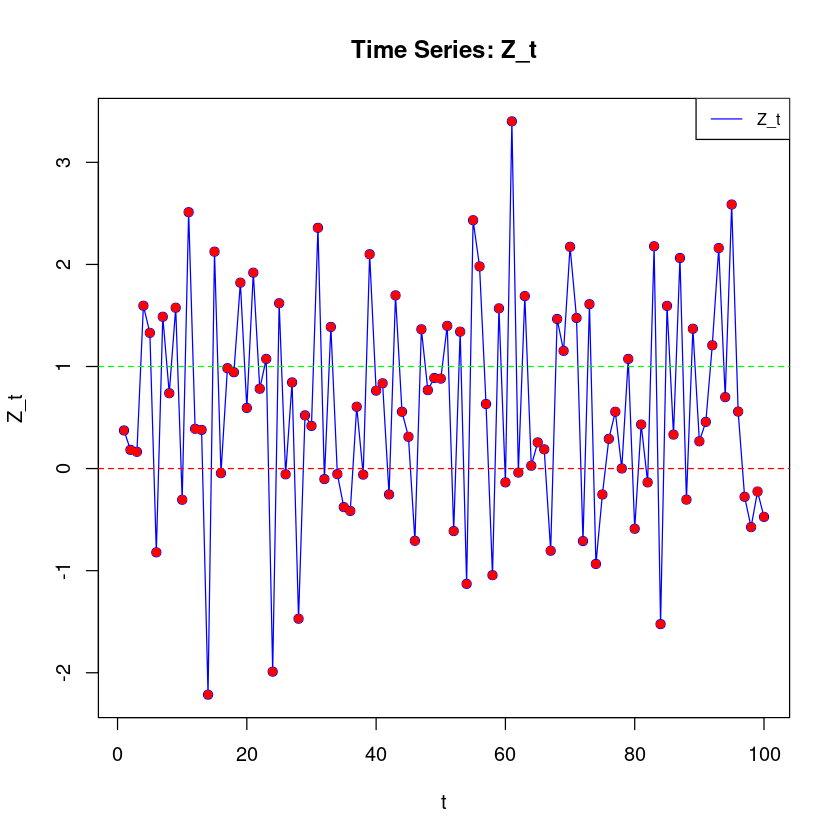

acf(Z)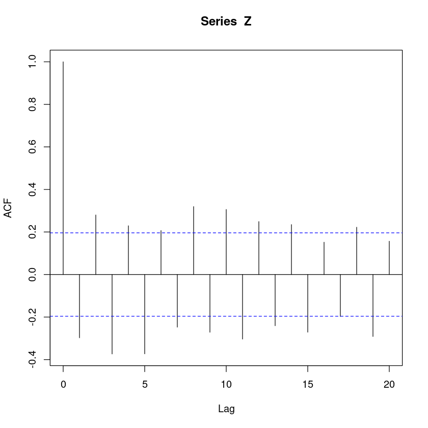

pacf(Z)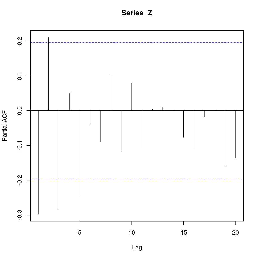

3

$ε_t$가 $WN(0, σ^2)$를 따를 때, 다음과 같은 확률과정 모형에 대하여 각 물음에 답하여라

\[Z_t − 0.8Z_{t−1} = ε_t\]

(1)

모형을 $ϕ(B)(Z_t − µ) = θ(B)ε_t$로 표현하고, $ϕ(B), θ(B)$ 그리고 $µ$를 명시하여라.

$(1-0.8B)Z_t = \epsilon_t$

$\mu-0.8\mu = 0 \rightarrow \mu = 0$

$ϕ(B)=1-0.8B$

$\theta(B) = 1$

$\mu=0$

(2)

모형은 AR(p), MA(q) 혹은 ARMA(p, q)모형 중 어느 것인가? p와 q도 함께 명시하여라.

AR(1)

(3)

ACF $ρ_k, k = 1, . . . , 5$를 계산하여라.

$lag=0, Cov(Z_t,Z_t)$ 를 구하자.

$\gamma_0 = [1+0.8^2 +0.8^4 +\dots ] \sigma^2=\dfrac{\sigma^2}{1-0.8^2}$

$lag=1$

	$\epsilon_t$	$\epsilon_{t-1}$	$\epsilon_{t-2}$	$\dots$
$Z_t$	1	0.8	$0.8^2$	$\dots$
$Z_{t-1}$	0	1	0.8	$\dots$

$\gamma_1 = [0+0.8 + 0.8^3 + \dots] \sigma^2 = \dfrac{0.8 \sigma^2}{1-0.8^2}$

즉

$\gamma_0 = \dfrac{\sigma^2}{1-0.8^2}$

$\gamma_1 = \dfrac{0.8\sigma^2}{1-0.8^2}$

$\gamma_2 = \dfrac{0.8^2\sigma^2}{1-0.8^2}$

$\gamma_3 = \dfrac{0.8^3\sigma^2}{1-0.8^2}$

$\gamma_4 = \dfrac{0.8^4\sigma^2}{1-0.8^2}$

$\gamma_5 = \dfrac{0.8^5\sigma^2}{1-0.8^2}$

$\rho_k = \dfrac{\gamma_k}{\gamma_0}$

$\rho_1 = \dfrac{\gamma_1}{\gamma_0}=0.8$

$\rho_2 = \dfrac{\gamma_2}{\gamma_0}=0.8^2$

$\rho_3 = \dfrac{\gamma_3}{\gamma_0}=0.8^3$

$\rho_4 = \dfrac{\gamma_4}{\gamma_0}=0.8^4$

$\rho_5 = \dfrac{\gamma_5}{\gamma_0}=0.8^5$

(4)

PACF $ϕ_{kk}, k = 1, . . . , 5$를 계산하여라.

$ϕ_{11}=\rho_1 = 0.8$

AR(1)모형이므로 $k \geq 2$이면 $ϕ_{kk}=0$이다.

(5) 다시…

위에서 구한 $ρ_k, ϕ_{kk}$ 의 상관도표를 그려라

##AR(1) phi=0.8
z <- arima.sim(n=1000, ##order=c(p,d,q) ARMA : d=0, AR : d=q=0
 list(order=c(1,0,0), ar= 0.8), #ar=ϕ1
 rand.gen = rnorm,
 sd = sqrt(1)) #분산
forecast::tsdisplay(z, lag.max=24)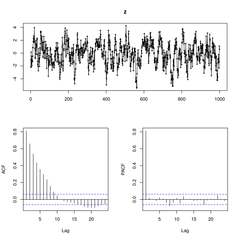

ACF그림은 지수적으로 감소하는 형태이고.
PACF는 h=1에서만 값이 존재하고 나머지는 다 0이다

4

다음의 모형에 대하여 다음 물음에 답하여라.

\[Z_t = ε_t − θ_1ε_{t−1} − θ_2ε_{t−2}, ε_t ∼ W N(0, σ^2)\]

(1)

자기상관함수(ACF) $ρ_h, h = 1, 2, . . .$를 구하시오.

$\gamma_k = Cov(Z_t, Z_{t-k}) = E[(ε_t − θ_1ε_{t−1} − θ_2ε_{t−2})(ε_{t-1} − θ_1ε_{t−2} − θ_2ε_{t−3})]$

lag=0

$\gamma_0 = (1+\theta_1^2 + \theta_2^2)$

1	- theta_1	- theta_2
1	- theta_1	- theta_2

lag=1

$\gamma_1 =-\theta_1 + \theta_1 \theta_2$

1	- theta_1	- theta_2
–	1	- theta_1

lag2

$\gamma_2 = -\theta_2$

1	-theta_1	- theta_2
–	–	1

$\rho_1 = \dfrac{\rho_1}{\rho_0} = \dfrac{-\theta_1 + \theta_1 \theta_2}{1+\theta_1^2 + \theta_2^2}$

$\rho_2 = \dfrac{\rho_2}{\rho_0} = \dfrac{-\theta_2}{1+\theta_1^2 + \theta_2^2}$

MA(2)모형이므로 k가 3이상이면 acf값은 다 0이다

(2)

부분자기상관함수(PACF) $ϕ_{11}, ϕ_{22}$를 구하시오.

$ϕ_{11}=\rho_1 = \dfrac{-\theta_1 + \theta_1 \theta_2}{1+\theta_1^2 + \theta_2^2}$

$ϕ_{22} = \dfrac{\rho_2 - \rho_1^2}{1-\rho_1^2}$

계싼복잡…생략..

5

$ε_t$ 가 $WN(0, σ^2)$를 따를 때, 다음과 같은 확률과정의 모형들에 대하여 각 물음에 답하여라. (단, (3)-(5)는 R을 이용하여, 각 모형을 따르는 10000개의 데이터를 생성한 후, acf, pacf 함수를 이용 한다.)

모형 1 : $Z_t − 9.5 = ε_t − 1.3ε_{t−1} + 0.6ε_{t−2}$

모형 2 : $Z_t − 0.6Z_{t−1} = 38 + ε_t + 0.9ε_{t−1}$

모형 3 : $Z_t = 26 + 0.6Z_{t−1} + ε_t + 0.2ε_{t−1} + 0.5ε_{t−2}$

모형 4 : $Z_t − 1.5Z_{t−1} + 0.7Z_{t−2} = 100 + ε_t − 0.5ε_{t−1}$

(1)

모형을 $ϕ(B)(Z_t − µ) = θ(B)ε_t$로 표현하고, $ϕ(B), θ(B)$ 그리고 $µ$를 명시하여라.

모형1

$(Z_t-9.5) = (1-1.3B + 0.6 B^2)\epsilon_t$

$ϕ(B)=1, θ(B)=(1-1.3B + 0.6 B^2), \mu=9.5$

모형2

$(1-0.6B)(Z_t - \mu) = (1+0.9B)\epsilon_t$

$\mu - 0.6 \mu = 38 \rightarrow \mu=38/0.4$

모형3

$(1-0.6B)(Z_t-\mu) = (1+0.2B +0.8B^2)\epsilon_t$

$ϕ(B)=1-0.6B, θ(B)=(1+0.2B +0.8B^2)$

$\mu-0.6\mu = 26 \rightarrow 0.4\mu = 26 \rightarrow \mu = 26/0.4=65$

모형4

$(1-1.5B+0.7B^2)(Z_t-\mu) = (1-0.5B)\epsilon_t$

$\mu - 1.5\mu + 0.7 \mu =100$

$\mu=500$

(2)

모형은 AR(p), MA(q) 혹은 ARMA(p, q)모형 중 어느 것인가? p와 q도 함께 명시하여라.

모형1 : MA(2)

모형2 : ARMA(1,1)

모형3 : ARMA(1,2)

모형4 : ARMA(2,1)

(5)

위에서 구한 $ρ_k, ϕ_{kk}$ 의 상관도표를 그려라

모형1

z1 <- arima.sim(n=10000,
 list(order=c(0,0,2), ma=c(1.3, -0.6)))
forecast::tsdisplay(z1, lag.max=24)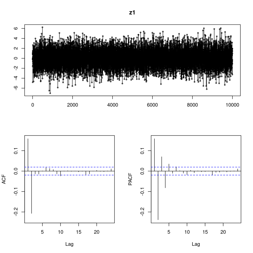

모형2

z2 <- arima.sim(n=10000,
 list(order=c(1,0,1), ar=0.6, ma=0.9),
 rand.gen = rnorm)
forecast::tsdisplay(z2, lag.max=24)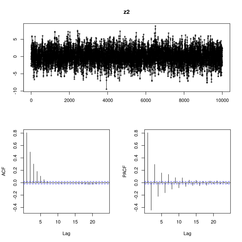

모형3

z3 <- arima.sim(n=10000,
 list(order=c(1,0,2), ar=0.6, ma=c(0.2,0.5)),
 rand.gen = rnorm)
forecast::tsdisplay(z3, lag.max=24)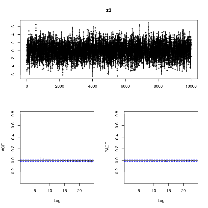

모형4

z4 <- arima.sim(n=10000,
 list(order=c(2,0,1), ar=c(1.5,-0.7), ma=-0.5),
 rand.gen = rnorm)
forecast::tsdisplay(z4, lag.max=24)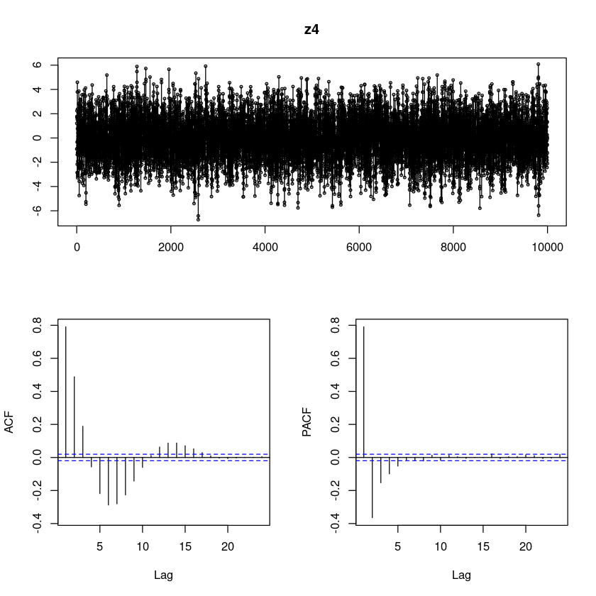

(3)

ACF $ρ_k, k = 1, . . . , 10$를 계산하여라.

모형1

acf_z1<-acf(z1,plot=FALSE)
acf_z1[1:10]


Autocorrelations of series ‘z1’, by lag

     1      2      3      4      5      6      7      8      9     10 
 0.158 -0.207 -0.014 -0.015  0.001  0.017  0.013  0.008 -0.014 -0.024

모형2

acf_z2<-acf(z2,plot=FALSE)
acf_z2[1:10]


Autocorrelations of series ‘z2’, by lag

     1      2      3      4      5      6      7      8      9     10 
 0.807  0.495  0.302  0.183  0.107  0.051  0.015  0.002 -0.003 -0.009

모형3

acf_z3<-acf(z3,plot=FALSE)
acf_z3[1:10]


Autocorrelations of series ‘z3’, by lag

    1     2     3     4     5     6     7     8     9    10 
0.796 0.637 0.382 0.229 0.138 0.086 0.059 0.038 0.027 0.016

모형4

acf_z4<-acf(z4,plot=FALSE)
acf_z4[1:10]


Autocorrelations of series ‘z4’, by lag

     1      2      3      4      5      6      7      8      9     10 
 0.791  0.488  0.189 -0.057 -0.219 -0.288 -0.281 -0.227 -0.143 -0.060

(4)

PACF $ϕ_{kk}, k = 1, . . . , 10$를 계산하여라.

모형1

pacf_z1<-pacf(z1,plot=FALSE)
pacf_z1[1:10]


Partial autocorrelations of series ‘z1’, by lag

     1      2      3      4      5      6      7      8      9     10 
 0.158 -0.238  0.070 -0.082  0.035 -0.011  0.021  0.002 -0.010 -0.017

모형2

pacf_z2<-pacf(z2,plot=FALSE)
pacf_z2[1:10]


Partial autocorrelations of series ‘z2’, by lag

     1      2      3      4      5      6      7      8      9     10 
 0.807 -0.443  0.296 -0.221  0.158 -0.163  0.135 -0.105  0.082 -0.083

모형3

pacf_z3<-pacf(z3,plot=FALSE)
pacf_z3[1:10]


Partial autocorrelations of series ‘z3’, by lag

     1      2      3      4      5      6      7      8      9     10 
 0.796  0.010 -0.349  0.071  0.158 -0.059 -0.052  0.026  0.023 -0.019

모형4

pacf_z4<-pacf(z4,plot=FALSE)
pacf_z4[1:10]


Partial autocorrelations of series ‘z4’, by lag

     1      2      3      4      5      6      7      8      9     10 
 0.791 -0.365 -0.153 -0.099 -0.052 -0.016 -0.017 -0.021  0.013 -0.017

6

다음과 같은 ACF를 갖는 가역성 조건을 만족하는 MA(1)과정의 모형을 구하라.

\[ρ_0 = 0, ρ_1 = \dfrac{1}{9} , ρ_k = 0, k ≥ 0\]

$Z_t = \epsilon_t + \theta \epsilon_{t-1}$

$acf(1) = \dfrac{\gamma_1}{\gamma_2} = \dfrac{\theta}{1+\theta^2} = \dfrac{1}{9}$

$\theta^2 - 9 \theta + 1 = 0$

$\theta = \dfrac{9 +- \sqrt{77}}{2}$

$\therefore \theta = \dfrac{9 - \sqrt{77}}{2}$

7

(R실습). 확률과정 $Z_t = 1 + 0.9Z_{t−1} + ε_t, t = 1, 2, . . . , 100$으로부터 시계열 자료를 생성한 후 다음을 수행하라. 단 $Z_0 = 10$의 값을 주고 $ε_t$는 $ε_t$ $∼_{i.i.d.} N(0, 1)$이다.

(1)

$\{Z_t\}$의 시계열그림을 그려라.

zt<-c()
zt[1]<-1+0.9*10+rnorm(1)
for(i in 2:100) zt[i]<-1+0.9*zt[i-1]+rnorm(1)
zt

11.6339448027521
10.0297491611439
10.48063483597
9.93642780128935
12.10806261555
10.2152209396991
13.7460677185397
12.4263586349121
14.2456440350337
13.8729153099666
13.8890374145228
13.9096357199169
11.8863371309684
12.9440758775657
13.5247886391223
12.7296586313629
11.4648254531922
11.283064858838
11.8156929303286
11.7448658878451
12.32448262803
13.1115048005427
13.8239208468079
11.3770837195393
12.3094831568635
12.7681316908829
11.1969801637485
11.7850096742986
12.0017396538599
10.6792160011758
11.2148693275543
10.6308609660893
9.91138476326052
10.621892845388
10.4522213240463
9.20987208077002
9.58604819929471
10.1583427398488
10.2700295381873
9.71201245009552
9.44366007729987
10.4158409321234
8.5872299494766
9.78917635247713
10.8963137494163
12.2103678903036
9.86578693146142
9.22172683986994
9.25190651171671
9.77490401630087
8.39829231775574
8.02288161790795
9.33096801713232
10.5626886258504
12.2178435406066
10.8323714373393
9.33311061289182
8.75520751151145
6.99380448839169
8.30691924800892
7.31415617895965
8.60162312019057
8.66022818106746
8.80057388980463
9.0651181702265
10.3675019024102
10.459871851365
9.48213366411919
10.4384121274965
11.2615099419654
11.4697170638735
10.0056820675572
10.2359996396427
11.4242893053008
12.6602103679228
12.7574603409234
11.8908574765488
11.1575316713236
12.0110929132003
11.9939485154955
12.4728230524616
10.2075419571772
9.38962144084908
10.4548676710282
9.72979326504712
11.2340144963607
11.3405372075702
9.80425419934968
8.20459976095349
8.20525882325441
7.26026421509633
5.76925419364217
6.41193936626902
6.62448446575856
7.46042237514119
5.42011565691056
6.02517355061036
6.41190471763322
7.87428239163398
8.70956639743375

plot(zt)

(2)

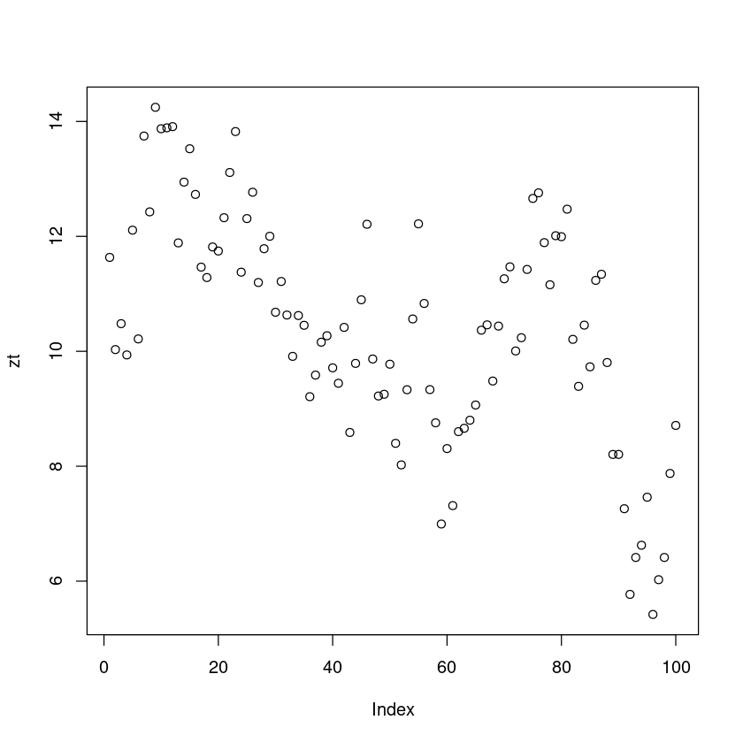
SACF, $\hatρ_h, h = 1, 2, . . . , 10$을 구하여 표본상관도표를 그려라

acf(zt)

acf(zt)$acf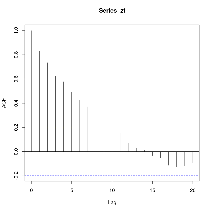

1
0.830045823110411
0.735129876073393
0.62619795113663
0.577356281418996
0.490427164682597
0.42649296433039
0.370321611649739
0.306248799055932
0.254412017586095
0.193156199329482
0.150250566238672
0.0713563901629154
0.029639995485257
0.0121346208843998
-0.0325772325466221
-0.0533571962757925
-0.112886388416267
-0.128414978937425
-0.119157092402368
-0.0926266728203544

(3)

SPACF, $\hat ϕ_{kk}, k = 1, 2, . . . , 10$을 구하여 표본상관도표를 그려라

pacf(zt)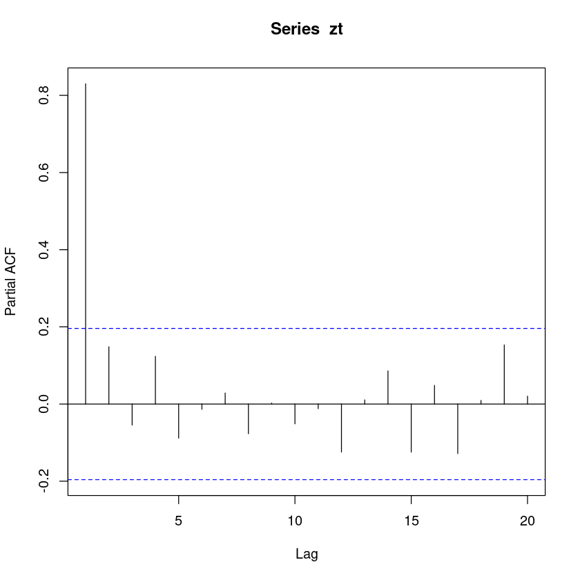

pacf(zt)$acf

0.830045823110411
0.148393107187214
-0.0546343362957735
0.123678558628976
-0.0883551477937624
-0.013798929554003
0.0286016292581917
-0.0769841241329633
0.00263703156357633
-0.0513306551749866
-0.012079285174621
-0.1246153113177
0.0108296561187292
0.0859635380334657
-0.124685817267623
0.0483698221700843
-0.128411011143925
0.00942969415608426
0.153161608224047
0.0205013651615918

(4)

$\{Z_t, Z_{t−1} \}$의 산점도를 그리고, 이 산점도와 $\hatρ_1$의 관계를 설명하여라

plot(zt,data.table::shift(zt,-1))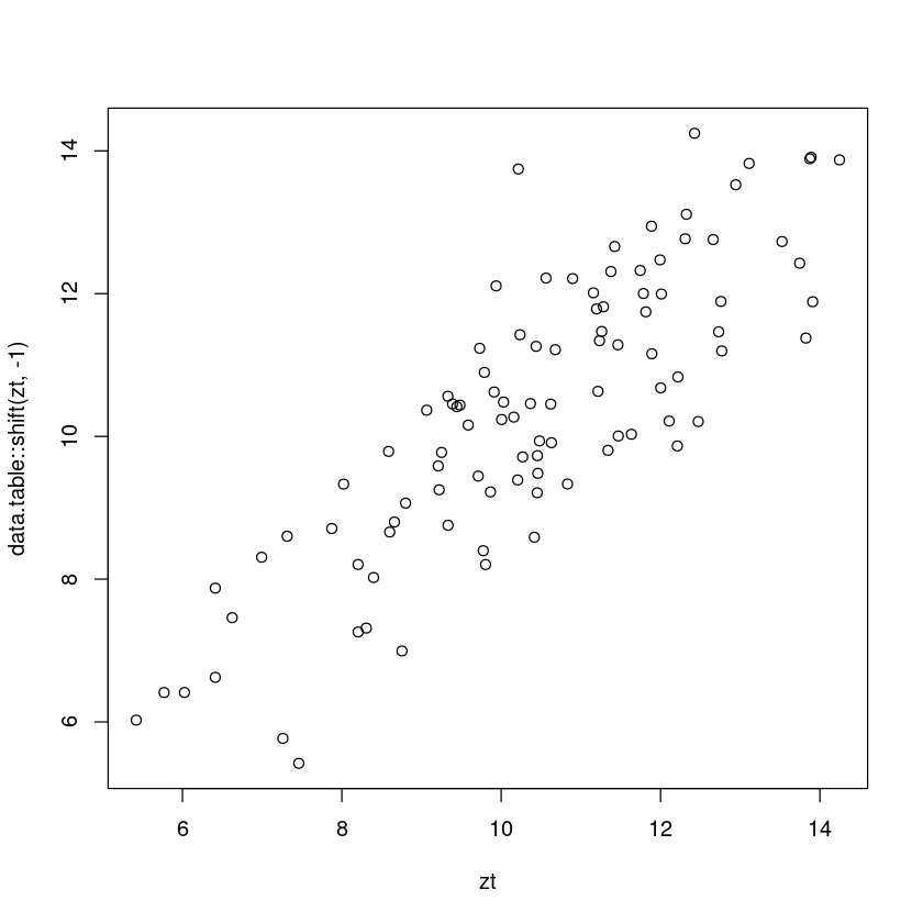

cor(zt,data.table::shift(zt,-1), use = 'pairwise.complete.obs')

0.834848419327365

(5)

$\{Z_t, Z_{t−2} \}$의 산점도를 그리고, 이 산점도와 $\hatρ_2$의 관계를 설명하여라

10.48063483597
9.93642780128935
12.10806261555
10.2152209396991
13.7460677185397
12.4263586349121
14.2456440350337
13.8729153099666
13.8890374145228
13.9096357199169
11.8863371309684
12.9440758775657
13.5247886391223
12.7296586313629
11.4648254531922
11.283064858838
11.8156929303286
11.7448658878451
12.32448262803
13.1115048005427
13.8239208468079
11.3770837195393
12.3094831568635
12.7681316908829
11.1969801637485
11.7850096742986
12.0017396538599
10.6792160011758
11.2148693275543
10.6308609660893
9.91138476326052
10.621892845388
10.4522213240463
9.20987208077002
9.58604819929471
10.1583427398488
10.2700295381873
9.71201245009552
9.44366007729987
10.4158409321234
8.5872299494766
9.78917635247713
10.8963137494163
12.2103678903036
9.86578693146142
9.22172683986994
9.25190651171671
9.77490401630087
8.39829231775574
8.02288161790795
9.33096801713232
10.5626886258504
12.2178435406066
10.8323714373393
9.33311061289182
8.75520751151145
6.99380448839169
8.30691924800892
7.31415617895965
8.60162312019057
8.66022818106746
8.80057388980463
9.0651181702265
10.3675019024102
10.459871851365
9.48213366411919
10.4384121274965
11.2615099419654
11.4697170638735
10.0056820675572
10.2359996396427
11.4242893053008
12.6602103679228
12.7574603409234
11.8908574765488
11.1575316713236
12.0110929132003
11.9939485154955
12.4728230524616
10.2075419571772
9.38962144084908
10.4548676710282
9.72979326504712
11.2340144963607
11.3405372075702
9.80425419934968
8.20459976095349
8.20525882325441
7.26026421509633
5.76925419364217
6.41193936626902
6.62448446575856
7.46042237514119
5.42011565691056
6.02517355061036
6.41190471763322
7.87428239163398
8.70956639743375
<NA>
<NA>

plot(zt,data.table::shift(zt,-2))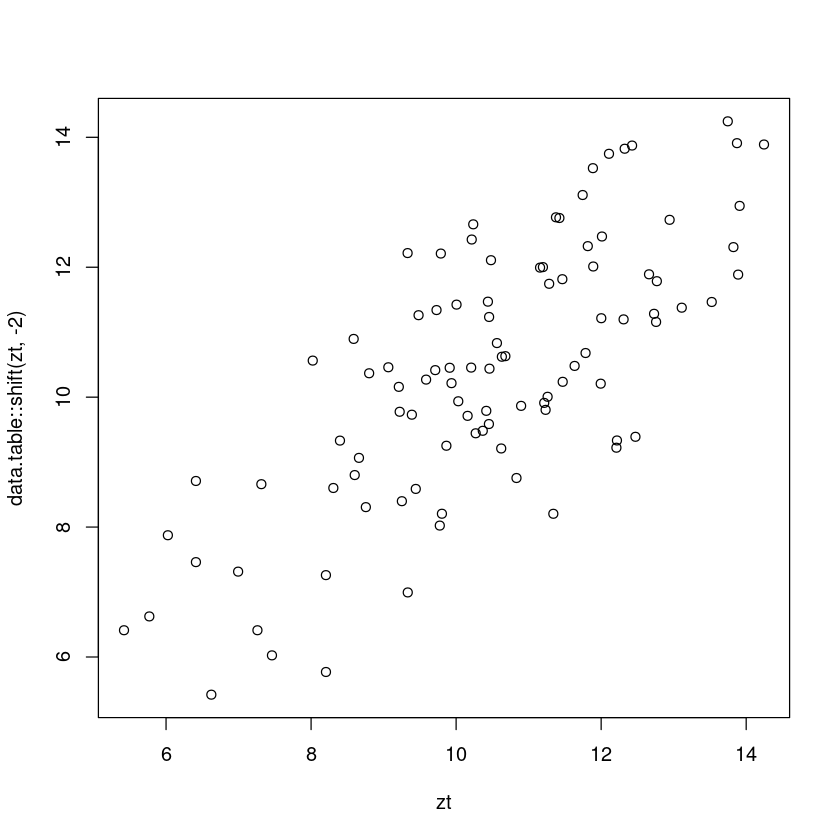

cor(zt,data.table::shift(zt,-2), use = 'pairwise.complete.obs')

0.745816184226449

	\(\epsilon_t\)	\(\epsilon_{t-1}\)	\(\epsilon_{t-2}\)	\(\dots\)
\(Z_t\)	1	0.8	\(0.8^2\)	\(\dots\)
\(Z_{t-1}\)	0	1	0.8	\(\dots\)